
This post is an elaboration on a project for a graduate course in Spatial Statistics. It focuses on the data science processes requried to build the data, explore it, and build a statistical model. However, it does not go into deep detail on the statistical methods used. If you are interested in a more technical write-up with some additional statistical techniques for analysis, please click here.
Intro & Disclaimer
Spatial statistics is a personal favorite subject. It is a powerful tool for modeling, but requires a thoughtfulness and creativity in how you approach crafting meaningful research questions, capturing the right data, and building of the model itself. The subject lends itself well to modeling of environmental phenomena, and we are fortunate to have free access to plenty of GIS data. This post will walk you through the steps I have personally used to approach the construction and analysis of a spatial statistics project analyzing wildfire patterns in Northern Arizona, a project I was a part of in graduate school which is where I will be drawing most of the content for this post.
NOTE
A quick disclaimer: I am not a wildfire expert, and this analysis is purely for educational purposes. Please do not use this analysis to inform any real-world decisions regarding wildfires. This post is mostly for fun and to give some accessible insights into some concepts in spatial statistics and the application of its techniques using publicly available data. That being said, I hope that this can provide some insight to the power of spatial statistics and how that power may be unlocked with the confluence of many different areas of expertise.
A Motivating Question
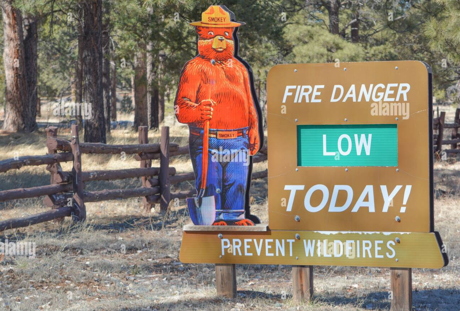
I grew up in Flagstaff, AZ, a heavily forested region of Northern Arizona. In fact, it's a part of the largest contiguous ponderosa pine forest in the world (seriously!). Naturally then, wildfire risk is of great concern to its inhabitants, particularly wildfires that grow large and out of control. I thought it would be interesting to explore spatial patterns of wildfires and analyze whether any available data could help build a risk model that can help predict whether wildfires are likely to grow large based upon where they start spatially, and to see if there are any environmental factors that legitimately contribute to this risk.
Before we begin, we must define a question or questions that we want to tackle. Arguably the most important step in building any analysis in statistics is the formulation of meaningful research questions. Research questions serve as the basis for the formulation of the data you pursue (through either direct measurement or proxy), as well as your approach to how you plan to analyze that data. It is also critical that your data, mathematical methods, and analysis are actually answering your questions (and not just providing a narrative), and that you are being thoughtful about the limitations of your data and methods.
Before we find our data and do exploratory analyses, we need to define a generalized question that can be meaningfully addressed.
Can we build a spatial model to predict the risk of large wildfires for a specified location? Can this model help determine what factors can contribute to elevated risk of large wildfires geographically?
This is a fairly open-ended question, but it provides us with some direction and goals to seek with this effort. The ultimate goal of finding answers to these questions is to build tools that can help inform wildfire prevention and mitigation strategies in the future. We want to keep these questions in mind as we compile our data, and be thoughtful about how we can use spatial statistical analyses to help us answer it.
Data Compilation
We will be using some pre-constructed datasets that can be referenced here. The data was compiled as detailed below and is reproducible using the data sources we'll detail, but a fair warning that it's a time-consuming task.
Wildfire Incident Data
For this type of problem, we know in advance that we will be seeking existing data, rather than collecting our own measurements. A topic for another time, but this is an important distinction; often methodoligies in how data is collected can impact what kinds of analyses can be actually done. So, since we aren't collecting our own data, and won't have any control over how or what data is captured, we will just need to take special care in understanding the data we do select.
We want to be certain that the data that is available for analysis will accommodate an appropriate spatial statistical analysis framework for answering our research questions in a meaningful way, and that the data within the dataset we choose is sensible for our goals. We want to study wildfires, but specifically wildfires that grow larger than some threshold and what factors may help to predict elevated risk of wildfires growing large depending upon where they start in some spatial location. So, our data must at least contain some coordinate location of a wildfire's origin, and its subsequent size in some measure.
Thankfully, we have public data available that should be useful to our cause. We'll be using the Wildland Fire Incident Locations dataset from the National Interagency Fire Center. In the next section, I'll describe in some more detail the exploratory data analysis that will help us inform our modeling approach, but first let's take a look at the foundation of the data we'll be using.
This dataset contains spatial point data indicating the origin of each wildfire recorded in the IRWIN database (since 2014), and includes many useful data attributes for each entry. The attributes from this dataset that are useful for our needs are the following.
xandy| Spatial coordinates in lat/lonIncidentSize| Size of the resulting wildfire in acresFireCause| Human, Natural, Unknown, UndeterminedFireDiscoveryDateTime| Date & time of incident reportingIncidentTypeCategory| WF (wildfire) or RX (prescribed burn)
This has the basics of what we need, plus some other factors of interest that we may not have previously considered, for example if the fire was deemed human/natural/undetermined in its cause.
All of our modeling will be done using R, and I'll make some notes about the code and packages used as we go along. Code snippets will be included along the way, but please note that they are only sketches and smaller chunks of larger scripts that generate the objects and artifacts that are used to build the model and visualizations.
NOTE
All of the code used for this article can be found in the public repo in the Reproducibility section at the end of this post. We will primarily be referencing the file Appendix_C_salce.Rmd in that repo for the code used in this analysis.
Wildfire Incident Data Exploration
The first step in the process of building an analysis is simple: look at the data!
As of November 2024, this original dataset contains over 300,000 recorded wildfire incidents across the entire United States since 2014. This is a lot of data to tackle, and we will need to subset it down to a manageable size and spatial region for our analysis.
We'll call our initial dataset wfigs_data_raw. Below is an interactive sample of the data that we will be using.
There are several steps that we can take to build a more manageable dataset, both spatially and intuitively. Let's first cover what techniques that we can use to filter our data down to the spatial region that we want to study.
NOTE
The code snippets shown in this post are simplified for clarity, and the order of operations in processing and subsetting data are presented to demonstrate a process that is starting from scratch and to help illustrate the concepts of the steps without skipping ahead. Plotting code is also omitted for brevity, but can be found in the public repo.
Subset Data Spatially - Arizona
The first step that we will take with this data is to clean up and subset the data spatially. To start, let's go over a quick summary of the spatial tools that we will be using in R.
Packages
sf| Simple Features for R: a powerful package for handling spatial data inR. It provides tools for reading, writing, and manipulating spatial data, as well as performing spatial operations and analyses.tigris| TIGER/Line shapefiles: AnRpackage that provides access to US Census Bureau TIGER/Line shapefiles, which allows loading of geographic geometry (as compatiblesfobjects) directly into ourRenvironment.dplyr| A grammar of data manipulation: A powerful package for data manipulation inR, giving us tools to filter, select, mutate, and summarize our data.ggplot2| A graphical package part oftidyverse: A widely used data visualization package inRthat we'll use to plot our data.
TIP
Every package I am using in this post is commonly used in spatial statistics in R and absolutely worth your time to learn! Even if you are not interested in spatial statistics, dplyr and ggplot2 are incredibly useful for general data manipulation and visualization.
We know that we have an overwhelming amount of data to work with, so the first step we will take in our data exploration will be to subset the data spatially down to just the state of Arizona. We may see some patterns in wildfire incidence that can help guide us to futher focus our analysis.
In the example R code below, we load in the necessary packages and create 'Simple Features' (sf) objects for the state of Arizona and its counties using the tigris package.
library(sf)
library(tigris)
library(dplyr)

# make state and county objects
arizona_sf <- states() %>% filter_state("arizona")
az_counties_sf <- counties(state = "AZ", cb = TRUE)
Projections
When working with spatial data, it is important to ensure that all spatial data is in the same Coordinate Reference System (CRS). This ensures that spatial operations and analyses are performed correctly and accurately.
One of the many powerful features of the sf package is its ability to easily transform spatial data between different CRSs. Once we have our spatial data loaded in as sf objects, we can use the st_transform() function to project our data to a common CRS.
Our coordinates in the attributes of our wildfire data are in the WGS84 coordinate system (EPSG:4326), which is a geographic coordinate system that uses latitude and longitude to define locations on the Earth's surface. However, for spatial statistical analysis, it is often more appropriate to use a projected coordinate system that preserves distances and areas more accurately.
All of the spatial data that we are using will be manually projected to the UTM Zone 12N coordinate reference system (EPSG:32612). This CRS has better spatial accuracy in the region of earth that contains Arizona, and will allow us to merge data from other sources that may use a different CRS by transforming them to this common CRS.
First we create our wildfire dataframe as an sf object, then we project it to UTM Zone 12N.
# note: wf_data_raw is the original wildfire data loaded in as a data.frame
# convert original wildfire data to sf object
wfigs_data_raw <- st_as_sf(wfigs_data_raw, coords = c("x", "y"), crs = "EPSG:4326")

# convert to UTM Zone 12N
wfigs_az_sf <- st_transform(wfigs_data_raw, crs = "EPSG:32612")
wfigs_az_sf <- st_intersection(wfigs_az_sf, arizona_sf)
Next we create our Arizona state and county sf objects, and project them to UTM Zone 12N as well.
# project to UTM Zone 12N
arizona_sf <- st_transform(arizona_sf, crs = "EPSG:32612")
az_counties_sf <- st_transform(az_counties_sf, crs = "EPSG:32612")
Once we have all of our spatial data projected and our sf objects created, we can use the st_intersection() function from the sf package to intersect wildfire data and the Arizona state boundary. This will allow us to filter our wildfire data to only include incidents that occurred within the state of Arizona.
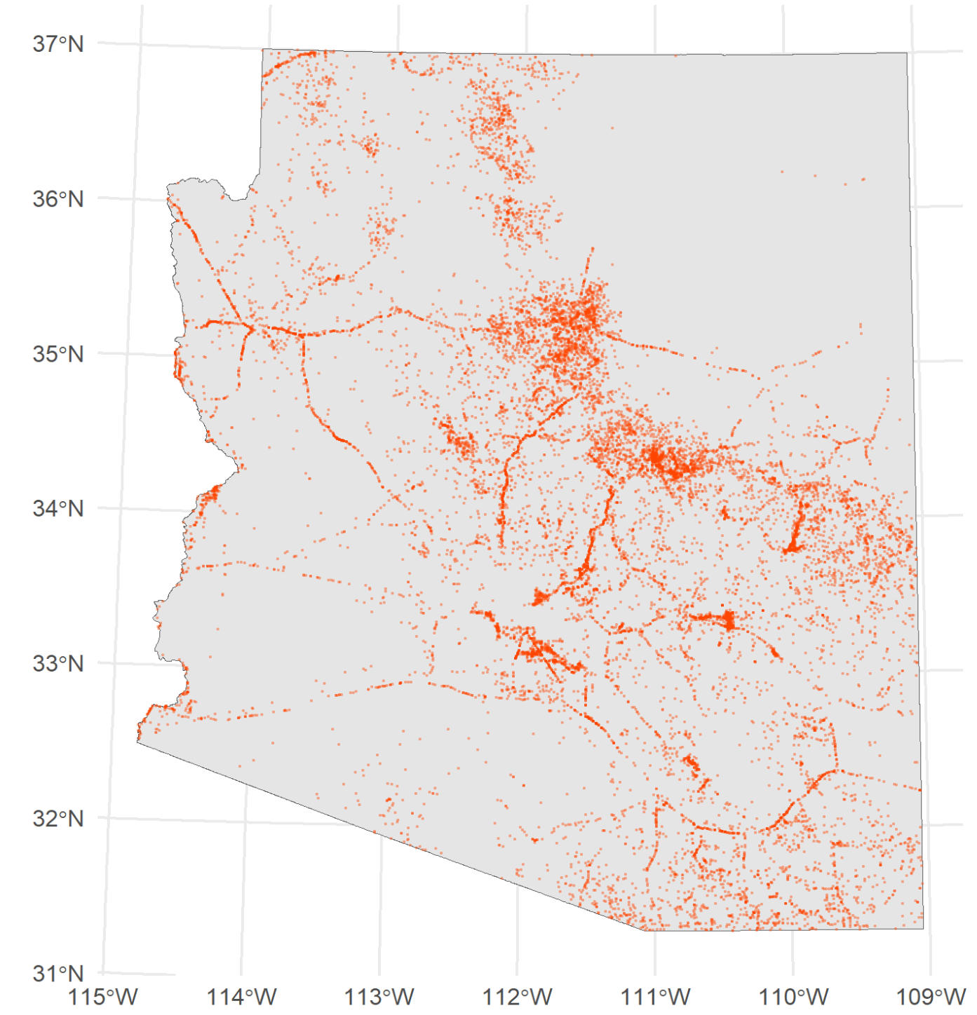
Our resulting dataset, wfigs_az_sf, now contains only wildfire incidents that occurred within the state of Arizona, which we have a first look at plotted below.
Subset Data - Human vs Natural Causes
Packages
tidycensus| An R package for accessing US Census data: A package that provides access to US Census Bureau data, allowing us to load in demographic and geographic data for our analysis.
After subsetting our data spatially to just Arizona, we still have a faily large dataset; about 18,000 wildfire incidents recorded since 2014.
The first dataset attribute that we can help to subset the data without much further exploration is the IncidentTypeCategory variable. This variable indicates whether the wildfire was a natural wildfire (WF) or a prescribed burn (RX). Since we are interested in studying wildfires that get out of control, we want to filter out any prescribed burns from our dataset. For those who may not be familiar, prescribed burns are intentionally set fires that are used as a land management tool to reduce the risk of larger wildfires.
Another attribute of interest is the FireCause variable, which indicates whether the wildfire was caused by human activity, natural causes, or is undetermined/unknown. As part of our data exploration, we want to see if there are any obvious differences in wildfire patterns between human-caused and natural-caused wildfires.
# subset to just wildfires (not prescribed burns)
az_fires_wf <- wfigs_az_sf %>% filter(IncidentTypeCategory == "WF")
# subset to human-caused and natural-caused wildfires
az_fires_wf_hum <- az_fires_wf %>% filter(FireCause == "Human")
az_fires_wf_nat <- az_fires_wf %>% filter(FireCause == "Natural")
Additionally, it may be useful to find some additional data that may supplement our visual explorations. In this case, we can find population density data that may help us understand if there are any spatial patterns in human-caused wildfires.
We will use the tidycensus package to load in population density data for Arizona at the census tract level. This package provides access to US Census Bureau data, and the get_decennial() function allows us to load in decennial census data for specific geographic regions. In this case, we are loading census data from 2010, however more recent data may be available by now.
library(tidycensus)
# load in population density data for Arizona
population_data <- get_decennial(
  geography = "tract",
  variables = c(population="P001001"),
  state = "AZ",
  year = 2010,
  geometry = TRUE
)
population_data$value[population_data$value==0] <- 1
population_data$variable <-  population_data$value/st_area(population_data$geometry)
names(population_data) <- c("GEOID","NAME","pop.density","pop.","geometry")
We then plot the log population density data with the human-caused and natural-caused wildfires overlaid in red, shown below.
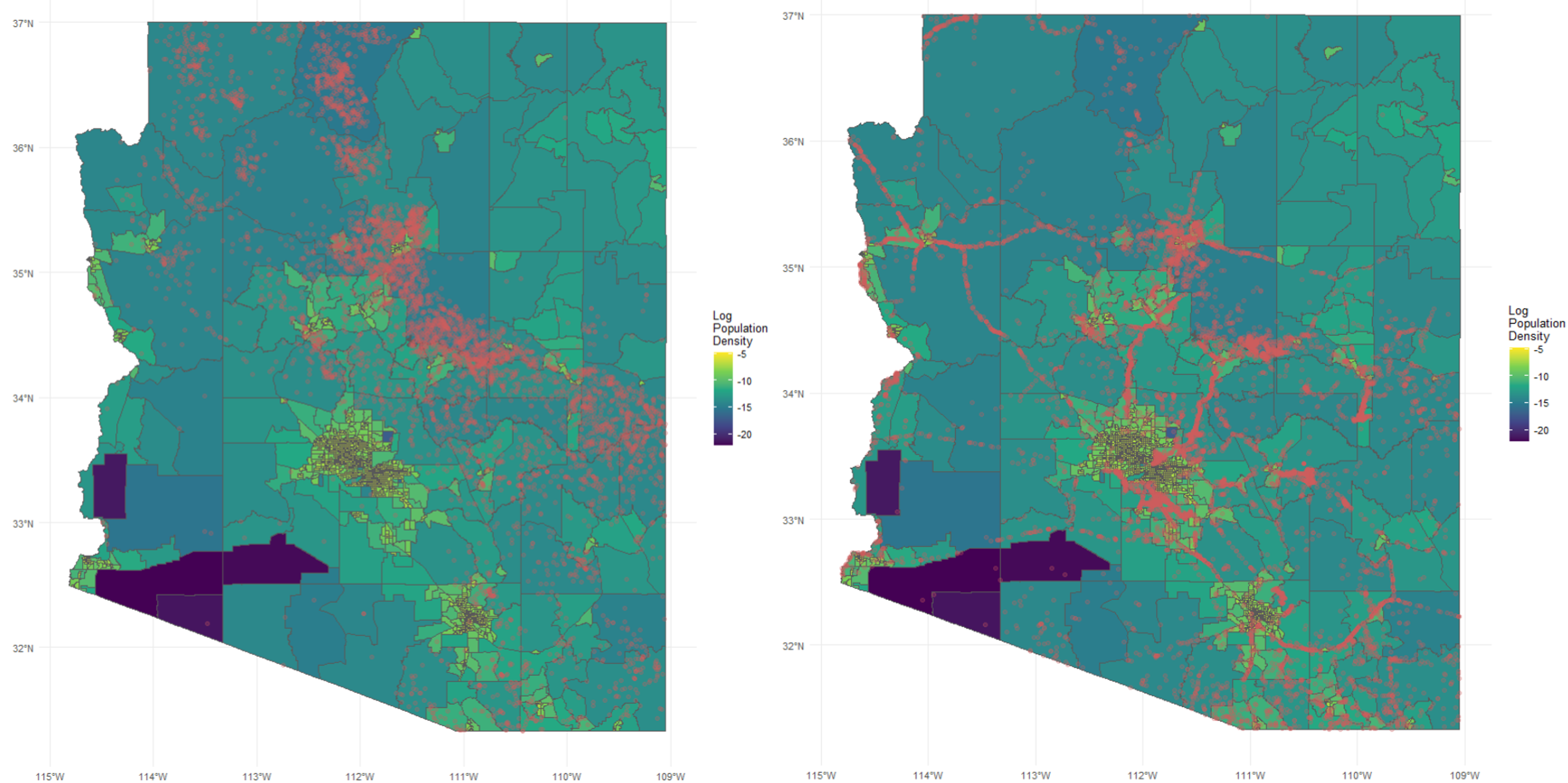
Population density and incidence, natural caused (left), human caused (right)
We can start to see some patterns emerging from our plots. Human-caused wildfires seem to be more concentrated in areas with higher population density, which makes intuitive sense. Natural-caused wildfires seem to be more evenly distributed across the state, with some higher concentration in certain areas of the state.
There is a striking pattern in the human-caused wildfires that seems to follow major roadways in Arizona. While this may not be too surprising, it is worth our attention to include in our modeling efforts to predict wildfire risk. We'll come back to this idea later (jump to that part of the post if you'd like) when we discuss "covariate" data, which is additional data for each wildfire incident that is used in a model that may factor into explaining large wildfire incidence.
Subset Data - AZ Counties, Coconino County
We are still working with a fairly large dataset, and we want to refine our data for analysis to something that isn't just manageable, but also useful to build a model that we can feel confident is answering our research questions before we apply it to new data. In this case, I wanted to focus on a region for which I have some intuition.
Now, it is not good practice to let any personal bias influence an approach to analysis, but as it happens there are good reasons to focus on a specific region, in this case. We can use our sf objects for Arizona counties to visualize where wildfires have been most prevalent in recent years.
az_county_intersections <- st_intersection(az_counties_sf,
  wfigs_az_sf[wfigs_az_sf$FireCause=="Human"|wfigs_az_sf$FireCause=="Natural",])

county_counts <- az_county_intersections %>%
  group_by(NAME) %>%
  summarise(count = n())

az_counties_with_counts <- az_counties_sf %>%
  st_join(county_counts, by = "NAME") %>%
  mutate(count = replace_na(count, 0))
We are using the st_intersection() function to find the intersection of our wildfire data with the Arizona counties, and then using dplyr functions to group the data by county and count the number of wildfires in each county. Note that we are omitting the "Unknown" and "Undetermined" wildfire causes here. Since we will be using data for our model that may help explain human vs natural causes, we want to focus on the incidents where we know the cause with some certainty.
We then join this count data back to our original county sf object to create a new sf object that contains the wildfire counts for each county. Then, we plot using ggplot2.

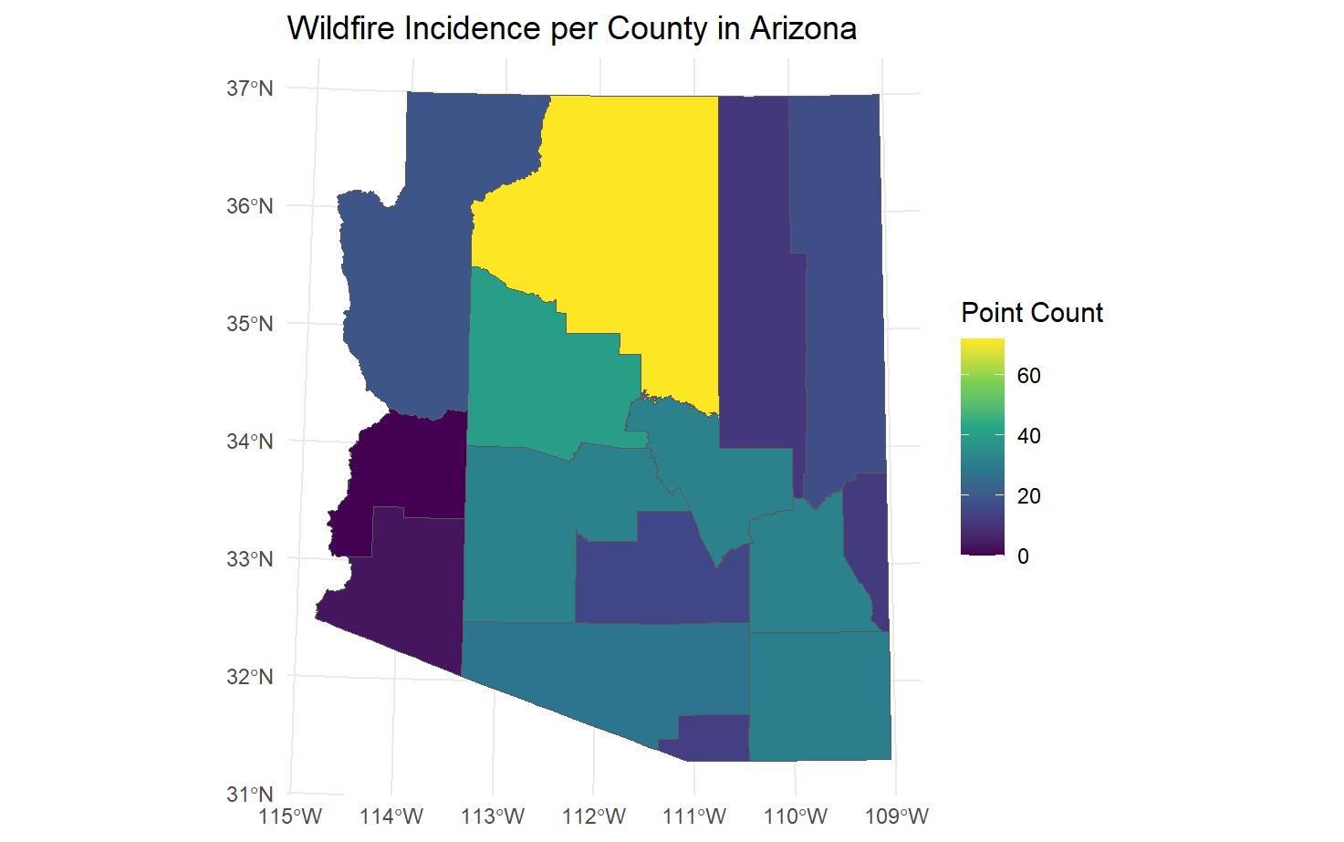
Wildfire Incidence per County in Arizona
As it happens, Coconino County (where my hometown of Flagstaff is located) has overwhelmingly more wildfire incidents that any other county in Arizona. As I mentioned earlier in this post, this is a heavily forested region, so it makes sense that wildfires would be so much more prevalent here.
Subset Data - Large Wildfires
There was some specific language in the original research question that has not yet been addressed. We are interested in building a model to predict the risk of large wildfires. So far, we have been looking at all wildfire incidents, regardless of size.
We have waited until this point to subset the data by size because had we subsetted earlier, we may have missed some important spatial patterns in wildfire incidence that could help inform our modeling approach. For example, if we had only looked at large wildfires from the start, we may have missed patterns of human-caused wildfires being concentrated near roads (again, more on this later).
(Short, 2014) (link) defines wildfire size using a classification system based upon the number of acres burned where class A, the smallest (0-0.25 acres), through class G, the largest (5000+ acres). Class F and G wildfires constitute the largest wildfires, so we will define a "large" wildfire as one that is greater than 1000 acres. We'll filter our data to only include wildfires that are greater than 1000 acres in size. Now we can have another look at the wildfire incidence by county in Arizona, this time only including large wildfires, to be sure that the spatial patterns we saw earlier still hold.
# fire size threshold
# FIRE_SIZE_CLASS = Code for fire size based on the number of acres within the
# final fire perimeter (A=greater than 0 but less than or equal to 0.25 acres,
# B=0.26-9.9 acres, C=10.0-99.9 acres, D=100-299 acres, E=300 to 999 acres,
# F=1000 to 4999 acres, and G=5000+ acres).
# class F and G fires
wf_size_threshold <- 1000
wfigs_az_sf$size_threshold <- as.integer(
  wfigs_az_sf$IncidentSize >= wf_size_threshold)
wfigs_az_sf_thresh <- wfigs_az_sf %>% filter(size_threshold==1)
We then rerun our county intersection and counting code from earlier, using wfigs_az_sf_thresh as our wildfire dataset.
Our earlier observation still holds; Coconino County has the most wildfire incidents in Arizona, even when only considering large wildfires.
We now have a very reasonably sized dataset to proceed with our analysis, with a total of 72 large wildfire incidents in Coconino County since 2014. Below is an interactive map of these large wildfire incidents in Coconino County, AZ, as well as other large wildfire incidents in Arizona for context. Note: the color scale is logarithmic to better visualize fire sizes.
Interactive Map of Large Wildfires in AZ
Link to full page interactive map (easier to browse)
Covariate Data: Human Activity & Environmental Factors
Now we'll shift into acquiring "covariate" data, which is data that can be used in our model to help explain wildfire risk. We can start by expanding on some ideas from patterns that we observed during our exploratory data analysis. Since our data has definition for human and natural-caused wildfires, we can start thinking about what factors may contribute to elevated risk of wildfire risk.
NOTE
Covariate data is any data that is not the primary variable of interest but may help explain or predict the primary variable of interest. In this case, the primary variable of interest is the risk that a fire starting at a particular point spatially will become large. In spatial statistics, covariate data can be used to build more accurate models by incorporating additional information about the spatial context of the primary variable. We may not always use all of the covariate data that we collect, but it's good practice to collect (and try to understand) as much relevant data as possible and then decide later which variables to include in our models.
Human Activity Data: Proximity to Roadways
One of the striking patterns we observed in our exploration was that human-caused wildfires seemed to follow major roadways in Arizona. That pattern was not as obvious for naturally caused fires, and based on our plots from the exploration, it's not immediately obvious that the any patterns hold for large wildfires specifically (whether they are human or naturally caused). However, it's a reasonable hypothesis that proximity to roadways may be a useful covariate for predicting wildfire risk; wildfires could be at an elevated risk of growing large if they are not accesbile by major roadways. That's one of the advantages of statistical modeling; patterns that may not be obvious to the naked eye can be revealed with statistics!
The tigris package also provides access to sf objects for roadways in Arizona. We can use the roads() function to load in road data for Arizona, and then use the st_nearest_points() function from the sf package to find the nearest point on each road to each wildfire incident. Each roads geometry has a corresponding classification code according to the Census Bureau, and we chose to include “Primary Roads” (S1100) and “Secondary Roads” (S1200) to be representative of what we will call “major” roads. Separately, we used “Vehicular Trail (4WD)” (S1500) roads to represent “remote” roads.
az_fips <- fips_codes %>%
  filter(state == "AZ") %>%
  pull(state_code) %>%
  unique()
# Get all counties in the state
az_counties <- counties(state = az_fips, cb = TRUE)
# Fetch roads for all counties and combine into one sf object
az_roads <- map_dfr(az_counties$COUNTYFP, function(county) {
  roads(state = az_fips, county = county)
  }) %>% st_as_sf()
# Filter for primary and secondary roads
az_rd_primary <- az_roads_sf %>%
  filter(MTFCC %in% c("S1100"))  # Primary  roads
az_rd_secondary <- az_roads_sf %>%
  filter(MTFCC %in% c("S1200"))  # Secondary roads
az_rd_4wd <- az_roads_sf %>%
  filter(MTFCC %in% c("S1500"))  # 4WD roads
The above code fetches road data for all counties in Arizona, and filters for primary, secondary, and 4WD roads and creates separate sf objects for each. Note that the fips_codes object is a predefined object in the tidycensus package that we loaded earlier, and contains the FIPS codes for all US states and counties. Reference the interactive map above (note you can filter layers to display the roadways).
wfigs_az_sf$distance_rd_primary <-
  st_distance(wfigs_az_sf, az_rd_primary) %>% apply(1, min)
wfigs_az_sf$distance_rd_secondary <-
  st_distance(wfigs_az_sf, az_rd_secondary) %>% apply(1, min)
wfigs_az_sf$distance_rd_4wd <-
  st_distance(wfigs_az_sf, az_rd_4wd) %>% apply(1, min)
We then use the st_distance() function to compute the distance (in units of distance for EPSG:32612 (metres)) from each wildfire incident to the nearest point on each of the three road types, and store these distances in our wildfire dataset.
wfigs_az_sf <- wfigs_az_sf %>%
  mutate(distance_rd_min_prisec = pmin(distance_rd_primary,
                                    distance_rd_secondary))
wfigs_az_sf <- wfigs_az_sf %>%
  mutate(distance_rd_min_all = pmin(distance_rd_primary,
                                    distance_rd_secondary,
                                    distance_rd_4wd))
wfigs_az_sf$distance_rd_min_isprisec <- as.integer(wfigs_az_sf$distance_rd_min_all ==
                                                     wfigs_az_sf$distance_rd_min_prisec)
We then use this distance to determine whether the nearest road to each wildfire incident is a major roadway (primary or secondary), or a remote road (4WD trail). This will provide us a binary covariate that we can use in our modeling efforts to predict wildfire risk based on proximity to major vs remote roadways, and we also have raw distance data, all of which could be useful as covariate data for our risk model.
Roadway Proximity Data - Quick Exploration
Using our thresholded wildfire data as well as different cuts of our original dataset, we can visualize the relationship between wildfire size and proximity to roadways. I'm omitting the code in this section, but the details can be found in the public repo.
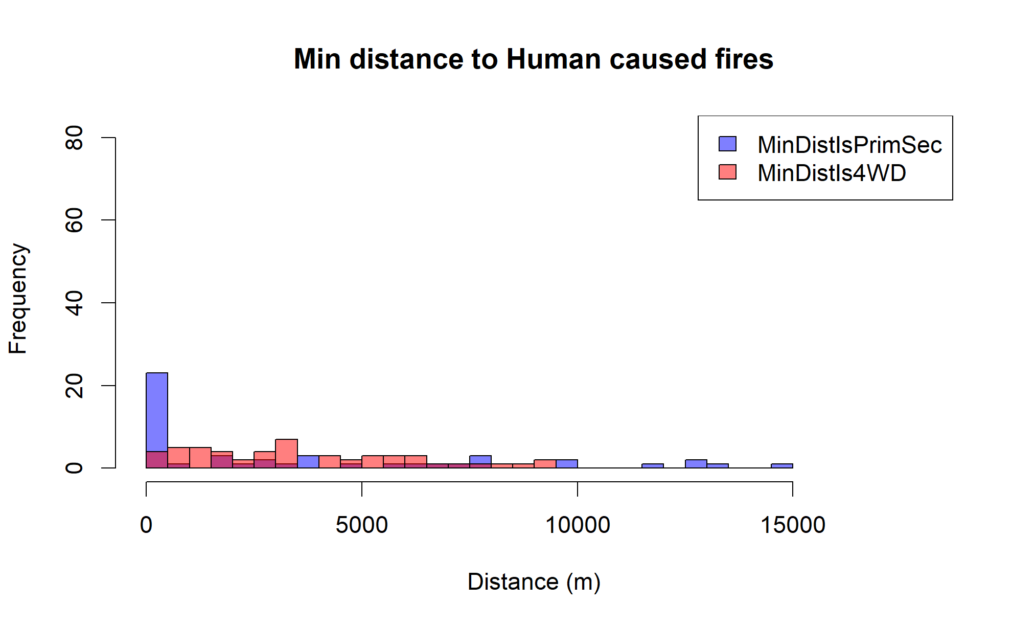
Looking at all wildfire data across Arizona (regardless of size), it's clear that there is a relationship between wildfire incidence and proximity to major roadways, and there is a new pattern we can now identify. First, let's look at a histogram of the human-cause wildfire incidence data binned by whether the nearest road is a major roadway (primary or secondary) or a remote road (4WD trail) and also by their distance. Note that the scale changes between the plots as we filter down data.
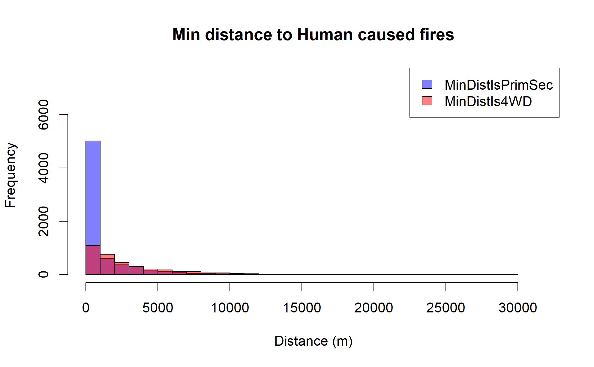
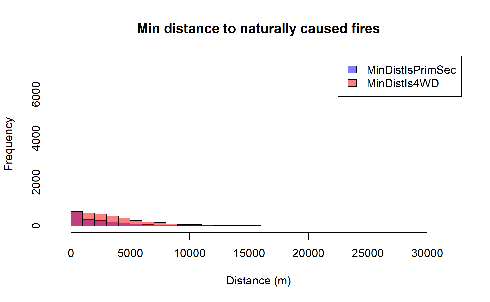
Clearly, human-caused wildfires are much more likely to be near major roadways, while naturally caused wildfires are somewhat more evenly distributed in proximity between major and remote roadways (but generally favoring more remote).
If we look at the same data for large wildfires only across the entire state, we see a similar pattern, but with some interesting differences.
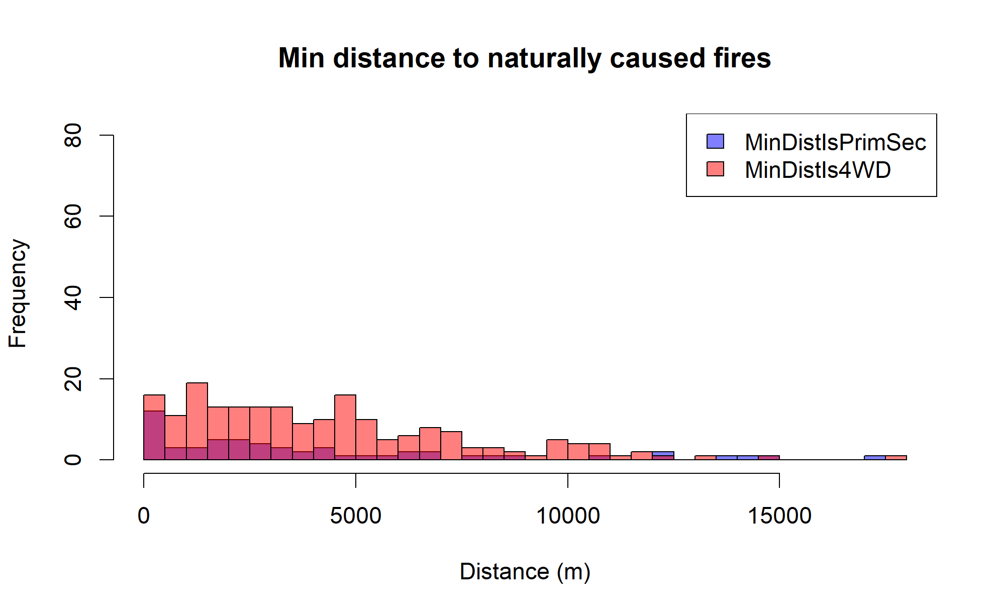
Large human-caused wildfires still show a strong preference for being near major roadways, but large naturally caused wildfires are generally much more remote.
Lastly, we want to look at just our thresholded wildfire data in Coconino County, since this is the dataset that we will be using for our modeling efforts.
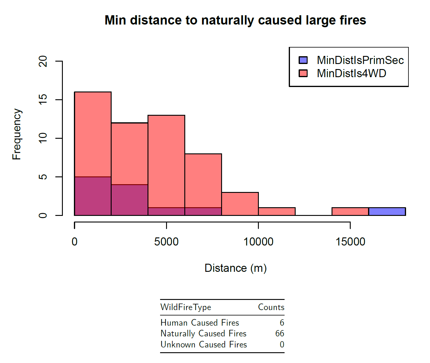
Naturally caused large wildfires in Coconino County tend to be more remote, which supports the trends we saw earlier, and makes intuitive sense as these are typically from lightning strikes. Overall, it seems that proximity to major roadways may be a useful covariate for predicting wildfire risk, so we will attempt to include this in our models.
Human Activity Data: Population Density
Population density may also be a useful covariate for predicting wildfire risk. We collected population density data earlier during our exploratory data analysis, and we can attempt to use this data in our modeling efforts as well. In general, we should expect that more human-caused wildfires will occur in areas with higher population density, but it's not immediately obvious how this will impact the risk of a wildfire growing large.
Since we are only using naturally caused wildfires in our modeling efforts, it's not immediately clear that population density will be a useful covariate at all. However, it's worth exploring and seeing if there is any relationship between population density and wildfire size. Also, if we later decide to expand the model to other regions and decide to include human-caused wildfires, population density may be a useful covariate. Refer back to the diagram here for a visualization of population density in Arizona.
Environmental Factor Data: Weather, Vegetation, Topography
For this portion of the data compilation, access to special tools like Digital Elevation Model (DEM) and National Land Cover Database (NLCD) was required in order to capture natural factors like percent slope, elevation, and vegetation cover. Data needed to be collected for each wildfire incidence location point using these separate tools, so it's difficult to reproduce with any new data. Some useful tools exist that could potentially capture this data better spatially like the terra package in R, which could be a worthwhile endeavor for future work.
Data at each wildfire incidence location point was extracted using a 1000-meter buffer to capture these characteristics because it helps us understand the landscape better and how it might influence fire behavior. A few example points are provided below.
Not all data was difficult to access though; we used the daymetr package to recover historical data on temperature and precipitation averages at each incident location, so this is something that could be more reliably reproduced with new wildfire incidence data.
Seasons
As another covariate to consider, we can also categorize each wildfire incident by the season in which it occurred. This may help us understand if there are any seasonal patterns in wildfire risk. We'll capture the season as a categorical variable with four levels: Winter (Dec-Feb), Spring (Mar-May), Summer (Jun-Aug), and Fall (Sep-Nov). This may be redundant in some ways, but sometimes more general categorizations can help capture patterns that more specific data may miss, and we are not obliagted to use it in our final model. We can use the function below as part of our model's equation when we start fitting the model to data.
get_season <- function(date) {
  month <- as.integer(format(date, "%m"))
  season <- case_when(
    month %in% c(12, 1, 2) ~ 1,
    month %in% c(3, 4, 5) ~ 2,
    month %in% c(6, 7, 8) ~ 3,
    month %in% c(9, 10, 11) ~ 4
  )
  return(season)
}
Statistical Modeling
Packages
spatstat| Spatial Point Pattern Analysis, Model-Fitting, Simulation, Prediction, and Simulation: A comprehensive package for spatial point pattern analysis inR. It provides tools for analyzing spatial point patterns, fitting spatial models, and performing spatial simulations.spmodel| Spatial Statistical Modeling: AnRpackage for spatial statistical modeling, providing tools for fitting spatial models to data and performing spatial predictions.
Before we begin building our statistical model, let's revisit our research questions to ensure that our modeling approach makes sense to answer our questions.
Can we build a spatial model to predict the risk of large wildfires for a specified location? Can this model help determine what factors can contribute to elevated risk of large wildfires geographically?
The modeling approach that we select should be a spatial model that can use a point spatially for its input, along with some supplemental covariate data for that point, and output a risk estimate for that location. Additionally, we want to be able to interpret the model in a way that can help us understand what factors contribute to elevated risk of large wildfires geographically.
TIP
As an aside, I want to emphasize the importance of being deliberate and clear about answering the research questions in a meaningful way. By extension, it is equally important to be thoughtful about the formulation of the research questions themselves. Statistical modeling is an incredibly powerful tool, but it is not a magic box that can answer any question. Research questions and statistical models really go hand in hand, and deficiencies in either can lead to misguided analyses and incorrect conclusions. So, we want to always keep the research questions in mind throughout the entire process, from data collection to model selection to interpretation of results.
Model Selection - Point Process
Selecting the appropriate statistical model to support our research questions is a critical step, but largely beyond the scope of this post, mostly because of the statistical background required to cover the process properly. However, I still wanted to cover some of high level reasoning that can give some insight into the inner workings of an appropriate model for this research question.
In this case, our data consists of points spatially representing large wildfire incident locations. This type of data is often referred to as "point pattern data", which are points that are assumed to be generated by some random process. For these types of data, we use point process models, which are a class of statistical models that are specifically designed to analyze and model the spatial distribution of points in a given area.
Defining "Risk" using a Binary Response Variable
First, we want to focus on the word "risk". In statistics, risk is often modeled using a binary response variable (using a "1" or a "0" to represent whether an event did or did not happen). Our data indicates locations where large wildfires have actually occurred, and we can treat them as "events" in our model (1 = large wildfire occurred). However we currently do not have data where large wildfires did not occur (0 = no large wildfire occurred).
Binary Response GLM Spatial Logistic Regression Model using Poisson Point Process
The advantage to using a binary response variable is that it allows us to model the probability of an event occurring at a given location using spatial logistic regression techniques (here's a fun StatQuest video about logistic regression). That is, our model will take points spatially along with corresponding covariate data as inputs, and it will output a probability (between 0 and 1) that a large wildfire will occur at that location with the input parameters. Hence, the model will predict "risk" of wildfire incidence.
Generating Background Points using Poisson Point Process
Since we don't currently have any in our data, we need to generate "non-event" locations where a large wildfire could have occurred, but did not. To do this, we can generate a set of background points using points randomly generated in our spatial domain (Coconino County) using a "constant intensity Poisson process". Essentially, we are generating points spatially according to a Poisson distribution called a "Poisson point process" with a known Poisson distribution parameter (intensity, represented by ) that describes the average number of points per unit area. Without going into too much detail, this technique gives us a viable way to fit a logistic regression model using the points where large wildfires did occur.
library(spatstat)

az_fires_wf_spglm_ppp <- as.ppp(az_fires_wf_nat)

background <- rpoispp((az_fires_wf_spglm_ppp$n) / area(as.owin(az_fires_wf_spglm_ppp)),
win = as.owin(coconino_sf))
This code snippet converts our naturally caused wildfire data in Coconino County to a spatstat point pattern object (ppp), and then generates background points using a Poisson point process with intensity equal to the number of wildfire incidents divided by the area of Coconino County. We can plot to see our incident data with the generated background points overlaid.
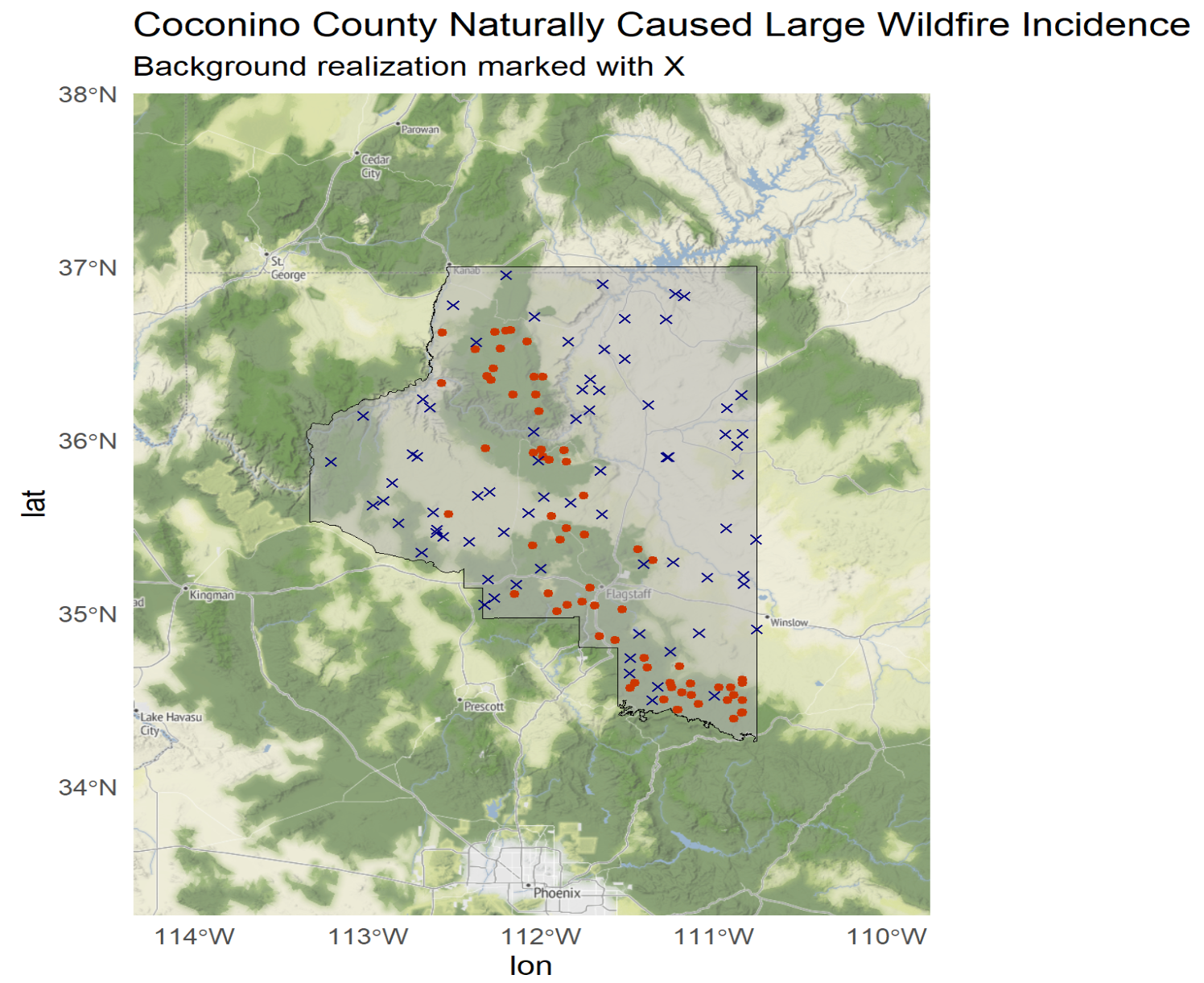
A side note here, we have converted back to EPSG:4326 due to some limitations in how we were able to capture covariate data for the wildfire incidents. More on this in the future work section
For each of these new points, we need to extract covariate data for the new generated background points since we don't have it yet. These steps are omitted; again, this requires some external tools, and future iterations of this study have opportunity to improve.
Fitting & Evaluating the Spatial Logistic Regression GLM (Generalized Linear Model)
The model we will be fitting is a spatial logistic regression model using a Generalized Linear Model (GLM) framework. The model can be expressed mathematically as follows:
Where:
- is the intensity of the point process at location ,
- is a vector of covariates at location ,
- is a vector of coefficients,
- is a spatial random effect,
- is the constant intensity parameter that we selected.
This is the form of the spatial logistic regression GLM that we will be fitting to our data. It has the form of a generalized linear model, only with an additional spatial random effect term. The inclusion of the spatial random effect is what makes this a spatial model; it accounts for spatial correlation in the data that is not explained by the covariate data alone. In other words, it captures spatial patterns that may be present in the data but are not accounted for by the covariates we have selected.
Once we have the covariate data captured for our background data, we can proceed with our logistic regression fit using the spmodel package.
Model Evaluation and Final Model Selection
All of the covariate and spatial covariance structure parameters for the final model were chosen based on a statistical selection process that is beyond the scope of the post, but generally involved fitting several models with different combinations of covariates and comparing their performance using metrics like AIC (Akaike Information Criterion) and BIC (Bayesian Information Criterion) in combination with a selected spatial covariance structure. Admittedly, this is a large omission as this is a very important part of the modeling process, but it would be difficult to cover properly without going into a lot of statistical detail.
Here is an example code snippet of the final model fit.
library(spmodel)

# model formula using selected covariates
spglm_formula <- Wildfires ~  distance_rd_min_isprisec + I(log(pop.density)) +
  Precipitation_Buffered * Temp_Min_Buffered + I(get_season(FireDiscoveryDateTime)) +
  mean_grass * mean_forest

#defining spatial covariance distribution
az_wf_spcov <- spcov_initial("wave")

# fitting the spatial logistic regression model
az_wf_spglm <- spglm(spglm_formula, data = model_data_sf,
                     family = binomial, spcov_initial = az_wf_spcov)
We're skipping several steps of statistical analysis here, but the above code snippet shows the general approach to fitting a spatial logistic regression model using the spmodel package. We define our model formula using selected covariates, specify a spatial covariance structure, and then fit the model using the spglm() function. Let's cover some important points about the model that was selected here.
Spatial Covariance Structure
The spatial covariance distribution is what differentiates a spatial model from a non-spatial model. As we touched upon already, the "spatial" part of the model captures behaviors in the data that are entirely spatial in nature, and cannot be explained by the covariate data alone, at least not in the covariate data that is available to us. The idea is that we have selected covariate data that helps to explain at least some of the wildfire risk at a selected location, but there may be other spatial factors at play that can't be captured by available covariate data in the model.
There is no one-size-fits-all approach to selecting a spatial covariance structure, and it often requires some trial and error to find a structure that fits the data well. We can think of the spatial covariance structure as a way to model the "leftover" spatial patterns ("residuals" in statistical terms) in the data that are not explained by the covariates, and depending on the covariate data we select, different spatial covariance structures may be more or less appropriate.
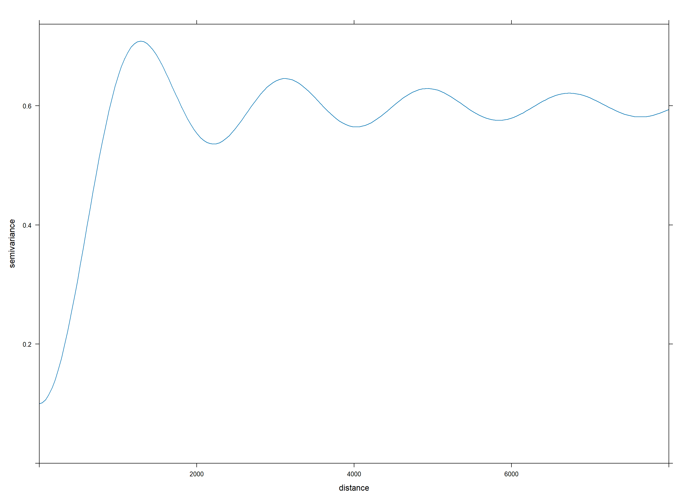
In this case, we selected a "wave" covariance structure, which is a structure typically used for spatial data that exhibits periodic behavior. This covariance structure is the best fit to model the "leftover" spatial patterns ("residuals") in the data that are not explained by the covariates.
We may proclaim that wildfire risk may exhibit some periodic behavior spatially, perhaps due to large wildfires' impacts on land immediately surrounding them and that burned forest is not likely to burn again soon after, with risk increasing again further away from the burned area. But this is largely speculative; it's rarely any exact science. The selection of the "wave" covariance structure was based on empirical performance rather than a strong theoretical basis, and can often be the case when selecting spatial covariance structures.
Covariate Selection
The covariates that were selected for the final model included proximity to major roadways, population density, precipitation and temperature (with an interaction term), seasonality, and vegetation cover (grass and forest), so for this model these factors were most useful for explaining wildfire risk in Coconino County.
Something worth noting...we didn't use all of the covariate data that we collected earlier! This is not an uncommon thing; we may collect data with a belief that it will improve the model performance, only to find out later that it has little to no effect on the model's predictive power. In this case, some of the environmental factors like elevation and slope were not selected for the final model, likely because they did not provide much additional information beyond what was already captured by other covariates.
Additionally, these covariates may not be the most useful for predicting wildfire risk in other regions, or even in Coconino County at different times. If we were to expand the modeled region, or applied the model to a different region (like a different county or state), the same covariate data may not be as useful to the model's predictive power. Extra covariate data that may have gone unused in this model may be more useful in other regions. So, it's always encouraged to collect as much relevant covariate data as possible, explore it and think it through, then evaluate which covariates to include in the model based on empirical performance.
Model Interpretation
One of our goals, and a goal that any good statistical model should strive for, is interpretability. We want for our model to give us insight about what factors contribute to elevated wildfire risk geographically, and how each factor influences the risk.
For this model, we can interpret the coefficients of the covariates in the model to understand how each factor influences wildfire risk. The resulting coefficients of the model we fit are as follows:
| Coefficient | Estimate | Std. Error | Pr(>z) | Interpretation |
|---|---|---|---|---|
| (Intercept) | -2.31282 | 7.91520 | 0.7701 | N/A |
| Proximity to major roadways | -1.32153 | 0.81237 | 0.1038 | Negative association with wildfire risk; proximity to roads is associated with lower risk |
| Population density | -0.10851 | 0.49135 | 0.8252 | Negative association with wildfire risk; higher population density is associated with lower risk |
| Annual Precipitiation | 0.06916 | 2.08641 | 0.9736 | Positive association with wildfire risk; greater annual precipitation is associated with higher risk |
| Average Annual Min Temperature | -1.12366 | 0.78317 | 0.1514 | Negative association with wildfire risk; lower minimum temperatures are associated with higher risk |
| Seasonality | 0.54990 | 0.37428 | 0.1418 | Positive association with wildfire risk; summer and fall seasons are associated with higher risk |
| Average grass coverage | 1.07408 | 1.74733 | 0.5388 | Positive association with wildfire risk; greater grass coverage is associated with higher risk |
| Average forest coverage | 1.30509 | 1.21915 | 0.2844 | Positive association with wildfire risk; greater forest coverage is associated with higher risk |
| Annual precipitation : Average Annual Min Temperature | 0.39667 | 0.52455 | 0.4495 | Positive association with wildfire risk; interactions of precipitation and temperature are associated with higher risk |
| Average grass coverage : Average forest coverage | 15.29506 | 9.16978 | 0.0953 | Positive association with wildfire risk; interactions of grass and forest coverage are associated with higher risk |
There is a lot that can be unpacked here, but the main takeaways I'd like to highlight are the following:
-
The "Interpretation" column provides a brief explanation of how each covariate influences wildfire risk based on the sign of the coefficient. We can't directly interpret the magnitude of the coefficients in a straightforward way because of the logistic regression framework, but we can say that positive coefficients are associated with increased wildfire risk, while negative coefficients are associated with decreased wildfire risk.
-
Terms with ":" indicate "interaction" terms, and while their coefficients cannot be directly interpreted, they represent the combined effect of two variables on wildfire risk.
-
The Pr(>z) column indicates the statistical significance of each coefficient. These are "p values" that you may already be familiar with from other statistical analyses. You may notice that none of the coefficients are statistically significant at a typical alpha level of 0.05. This does not necessarily mean that the covariates are not useful for predicting wildfire risk! Keep in mind that this model was selected based on an objective model performance evaluation process rather than statistical significance of individual coefficients.
-
There are many reasons why no coefficients are statistically significant, including the limited size of our dataset (only 66 naturally caused large wildfires in Coconino County since 2014), multicollinearity between covariates, and other factors. Clearly the influence of one covariate on its own does not seem to overwhelm the influence of other covariates, but together they provide our best predictive power for wildfire risk in this region. I'll leave it to the reader to rationalize what the covariate interpretations (or maybe there is no reasonable explanation to their signs at all). This is where we reach the confluence of statistics and domain expertise, and I am not a wildfire domain expert. Collaboration with domain experts can really help rationalize insights into the results of statistical models. For me, it's the best part of applied statistics; you get to work with experts in other fields to help make sense of the results of your analyses and learn more about the subject you're researching.
-
To reiterate on an earlier point, the covariates selected for this model may not be the most useful for predicting wildfire risk in other regions, or even in Coconino County at different times. If we were to expand the modeled region, or applied the model to a different region (like a different county or state), the same covariate data may not be as useful to the model's predictive power. Extra covariate data that may have gone unused in this model may be more useful in other regions. This process has given us a good framework for building spatial wildfire risk models, and as we expand to other regions, we can apply our knowledge from this model to help guide our covariate selection and model fitting efforts.
-
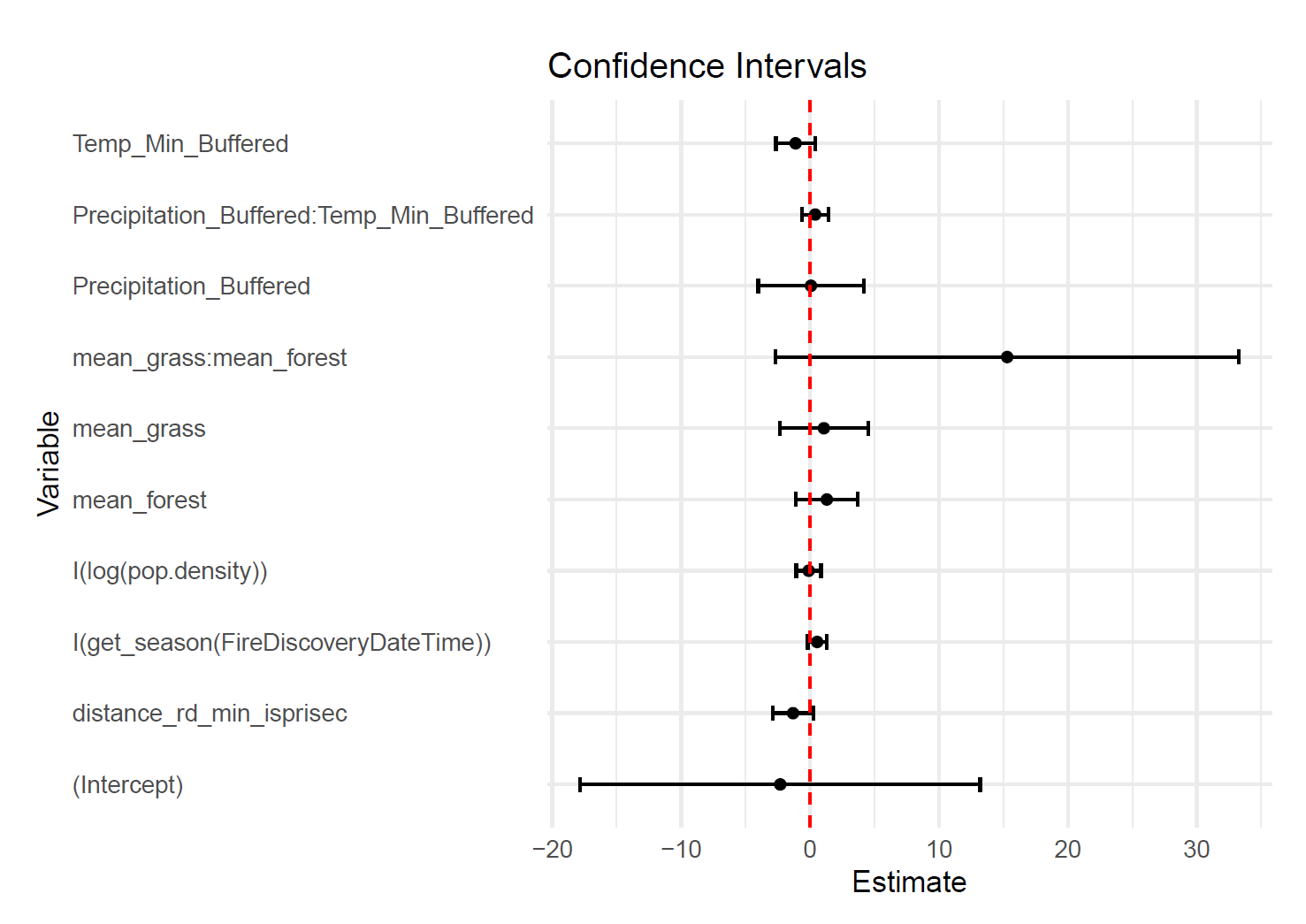
It's important to consider the confidence intervals of the model coefficients. The figure shown is the 95% confidence intervals (CI's) for the model coefficients. All of the CI's cover zero, that is that the confidence interval includes zero, indicating that it is feasible that the "true" parameter is actually zero. In other words, based on this data it's possible that none of these covariates actually can explain wildfire risk. See this article for more detail about confidence intervals.
Model Predictions
Now that we have fit our spatial logistic regression model, we can use it to make predictions about wildfire risk at new locations.
First, we need to create a grid of locations over Coconino County where we want to make predictions. We can then use the predict() function from the spmodel package to make predictions at each location in the grid.
# Create a grid of points
grid <- st_make_grid(coconino_sf, n = c(20, 20), what = "centers")
# Convert the grid to an sf object
grid_sf <- st_sf(geometry = grid)
# Filter points to keep only those inside Coconino County
coconino_grid <- grid_sf[coconino_sf, ]
# If you need exactly 200 points, you can sample from the resulting grid
coconino_grid_n <- coconino_grid %>%
  slice_sample(n = 400)

prediction_grid <- cbind(st_drop_geometry(coconino_grid_n), st_coordinates(coconino_grid_n))
prediction_grid$FireDiscoveryDateTime <- ymd_hm("2023-12-31 12:00")
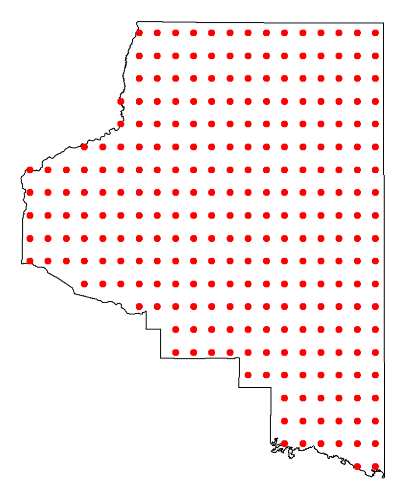
For our prediction grid, we are using a 20x20 grid of points over Coconino County, and then sampling 400 points from that grid to use for predictions. We also need to add a date to each point in the grid, since some of our covariates are time-dependent (like seasonality).
Next, we need to extract covariate data for each point in the prediction grid, similar to how we did for the wildfire incidents and background points earlier. Again, this requires some external tools, and future iterations of this study have opportunity to improve.
Once we've collected the covariate data for each point in the prediction grid (which we have stored in az_prediction_grid_sf), we can make predictions using our fitted model.
az_wf_predict_spglm <- predict(az_wf_spglm, type = "response", se.fit = T, newdata = az_prediction_grid_sf)
az_prediction_grid_sf$predict_bin_spglm <- az_wf_predict_spglm$fit
predict_plot <- st_transform(az_prediction_grid_sf, crs = 4326)

#national forest geometry for plots
naz_nf_plot <- st_transform(naz_forests_sf, crs = 4326 )
We use the predict() function to make predictions at each point in the prediction grid, specifying type = "response" to get predicted probabilities, and se.fit = T to also get standard errors for the predictions. We then store the predicted probabilities in a new column in our prediction grid dataset.
Finally, we can visualize the predicted wildfire risk over Coconino County using a heatmap.
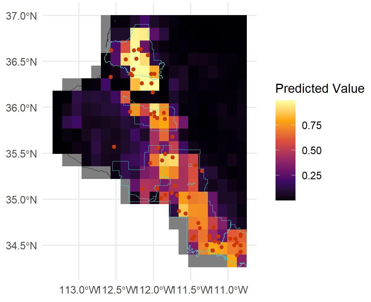
National forests are outlined in dark green. The heatmap shows the predicted probability of a large wildfire occurring at each location in Coconino County, with warmer colors indicating higher risk.
This animation shows how the predicted wildfire risk surface changes as we sweep through different levels of annual precipitation from -10% to +10%, holding all other covariates constant. We're only really demonstrating the model's prediction capabilities here, but this type of analysis could be useful for understanding how changes in environmental factors like precipitation can influence wildfire risk geographically.
Conclusions
The goal of building this spatial logistic regression model is to provide a tool for predicting wildfire risk geographically, and to help understand what factors contribute to elevated wildfire risk. In practice, a model like this could be used by land management agencies, firefighting organizations, and policymakers to inform decision-making related to wildfire prevention and mitigation (e.g., resource allocation, public awareness campaigns, land use planning).
But to reiterate a point from early in the post, please do not use this one! Our model is just a proof-of-concept that uses limited data for a specific region. More data, validation, and refinement would be needed to create a reliable and accurate wildfire risk prediction model for practical use. Models that are used in practice for wildfire risk prediction are typically built using much larger datasets, more sophisticated modeling techniques, and extensive validation processes, but this process gives a peek behind the curtain for the basics of how they are built.
Future Work & Improvements
We have touched on several areas where future work and improvements could be made to enhance the model's performance and reliability. Here are some key areas for future work:
Data Collection & Covariate Improvements
Now that we have a basic framework for building a spatial wildfire risk model, there are several areas where we can improve the data collection and covariate selection process to enhance the model's performance. Below are some areas that I consider to be the most impactful for future work, with the order roughly indicating priority.
Use of terra Package
Arguably the biggest limitation of the current framework is the external tools required to capture covariate data for wildfire incidents and background points. If we were able to access data like terrain, vegetation, and weather in a raster format, we could use the terra package in R to extract covariate data directly within the R environment. This would allow much greater flexibility in generating new background points and prediction grids, as we would be able to extract covariate data for any spatial location without relying on external tools. This flexibility would greatly enhance the reproducibility of the modeling process and allow for easier expansion to new regions and datasets.
terra| Spatial Data Analysis: An R package for spatial data analysis, providing tools for reading, writing, manipulating, and analyzing raster and vector spatial data. See rspatial.org for more info.
The raster data can be collected from various sources like USDA Forest Service, USGS Earth Explorer, NASA Earthdata, and Google Earth Engine.
Automation (API backend)
For this to be a model that could be used in practice, we should automate the data collection and model fitting process. This could be done by building an API backend that can handle data collection, model fitting, and prediction generation automatically. The backend API could be built using frameworks like Flask or FastAPI in Python, or Plumber in R, and could source live data from our original Wildland Fire Incident Locations dataset, and relevant sources like NASA FIRMS for wildfire incidents, NOAA for weather data, and other relevant sources for covariate data. The goal would be real-time updates to the model as new wildfire data becomes available, and would make it easier to deploy the model for practical use.
Projection Consistency
Additional effort should be made, particularly with the use of the terra package and the buildout of backend data, to establish projection consistency throughout the entire modeling process. One of the limitations of the current framework is the need to switch between different coordinate reference systems (CRS) at various points in the process, like use of external tools to capture covariate data. This can introduce errors and inconsistencies. Establishing a consistent CRS throughout the entire process, namely structured in the backend data, would help to mitigate these issues and improve the reliability of the model.
More Comprehensive Wildfire Data
It's reasonable to assume that our current model's performance is limited by the size and scope of the wildfire data used for training. We only used naturally caused large wildfires in Coconino County since 2014, which is a relatively small dataset. Expanding the dataset to include more wildfire incidents, both in terms of geographic scope (e.g., additional counties, other states with comparable wildfire risk profiles) and temporal scope (e.g., more years of data), could help to improve the model's performance and generalizability. Additionally, including human-caused wildfires could provide a more comprehensive view of wildfire risk (although this would require careful consideration of how to model the influence of human activity on wildfire risk).
Additional Covariates
The addition of more covariate data can help to unlock better predictive power for the model, and is an open area for future work. Some ideas to consider:
- Lightning strike data
- Wind speed and direction data
- Drought indices
- Fuel load data
- Prescribed burn data / distance to prescribed burns
- Human activity data (e.g., land use, recreational areas)
- More detailed vegetation data
- Soil moisture levels
- Historical wildfire suppression efforts
Other modeling approaches
This is not the only modeling approach that could be used for predicting wildfire risk. Other spatial modeling techniques, like machine learning approaches (e.g., random forests, gradient boosting machines) or Bayesian spatial models, could be explored to see if they provide better predictive performance or interpretability.
This post originated from a final project for a graduate course in spatial statistics, and my teammates provided two other approaches to modeling wildfire risk that may be worth exploring further in a more technical post that can be found here.